This report describes a technique to measure the numerical precisions required for correct execution of a real world program.
It identifies cases where the chosen precision is either inadequate or unnecessarily high, and for any chosen set of precisions, it finds the statements where the chosen precision is inadequate and computation breaks down.
The required precisions are measured to a resolution of 1 mantissa bit, and may be measured separately for each kind of real number which has been used.
Most high performance computers (HPCs) use 4 and 8 byte IEEE numbers with 23 and 52 mantissa bits. These number formats were defined in 1985, and the technique described can measure whether they are still appropriate for modern HPC systems.
More importantly, a large proportion of the resources of an HPC are used to move data between processors. It may be possible to improve the efficiency of HPCs by transferring only the number of bits required for safe and correct program execution.
10 and 16 byte real numbers are usually available in HPCs. FPGAs and GPUs are used in high performance computing, and these may have restricted precision, or, in the case of FPGAs, may use number formats with unusual precisions. The technique may easily be extended to measure where these should or should not be used.
The technique is applied to Fortran programs, and is applicable to programs in all languages which support variables of derived types and overloading of operators. It is applied here to two small sample programs.
For publication of this work, and references to related work, please see Collins J. 2017, Testing the Numerical Precisions Required to Execute Real World Programs", IJSEA Vol 8, No 2, March 2017. Attention is drawn in particular to the work of Andrew Dawson and Peter Düben at The Department of Atmospheric, Oceanic and Planetary Physics, University of Oxford.
All REAL and COMPLEX variables and Fortran parameters (Named constants) in the program under study are changed to objects of derived types which emulate the real numbers. This change is made automatically by a software engineering tool, and affects the declarations of the variables and a very small number of special cases in the executable code. For example, the declaration
REAL :: x
is changed to
TYPE(em_real_k4) :: x
Note that the original declaration may be written in many different ways and with arbitrary use of white space. The software engineering tool must recognise all equivalent declarations and make the appropriate change, as described here.
The program code contains arithmetic expressions, for example, a = b * c . The compiler has no rule to specify what the arithmetic operator * is to do with objects of the derived type em_real_k4. The rules are specified by overloading the arithmetic operators. The overloads are written in a Fortran module which is referenced in every top-level compilation unit. The reference is made by inserting the statement:
USE module_emulate_real_arithmetic
The insertion is made automatically by the software engineering tool. Each overload is made by calling a Fortran subroutine which carries out the overloaded operation.
The emulated real and complex types each contain a single component of the corresponding native type. Thus, for example, the type em_real_k4 contains a component of the native type REAL(KIND=kr4) where the integer kr4 is the kind value for a 4-byte IEEE number. The emulated types used in the present study are shown here.
The changes in precision are made in the functions and subroutines which overload the arithmetic. For example, the overload for multiplication of two 4-byte IEEE real numbers is shown here.
Within each function or subroutine which overloads the arithmetic, the change in precision is made by calls to one of the functions experiment_4 for 4-byte real numbers, experiment_8 for 8-byte real numbers or for experiment_x4 or experiment_x8 for the corresponding complex numbers. These functions round the mantissa of the emulated real number to a specified number of bits. Note that the functions round the arguments. They do not simply truncate them because this would cause a systematic bias in the result. The rounding function is called both before and after each arithmetic operation to prevent additional precision in values from I/O statements or constants in the code from entering the computations. The code of experiment_4 is shown here.
Additional functions could easily be added to round 10 and 16-byte real numbers.
A large number of overloading functions and subroutines must be included in the module module_emulate_real_arithmetic. Sub-programs are needed to overload simple assignment, the unary operators + and -, the arithmetic operators +, -, *, / and **, and the relational operators ==, /=, >, <, >= and <=. For the dyadic cases, these must be supplied for all combinations of emulated 4-byte and 8-byte real variables and the corresponding complex variables, with emulated 4-byte and 8-byte real variables, the corresponding complex variables, 4 and 8-byte real literal numbers, the corresponding complex literal numbers, and with 1, 2, 4 and 8-byte integer numbers. Overloads must also be supplied for all of the Fortran intrinsic functions and subroutines which operate on real and complex numbers. The codes of many of these sub-programs are closely similar, and programs were written to generate them automatically.
There are a number of additional changes which must be made to a program when the arithmetic is emulated. Most of these, except for the changes to parameter and data specifications, are infrequent, but they must be handled by the software engineering tools if the entire process is to be automatic. They are:
Changes to the values specified for Fortran parameters: Fortran parameters are compile-time constants. Real and complex Fortran parameters are converted to objects of the corresponding emulated types. The values must also be converted as described here;
Changes to real and complex data specifications: The values specified in data statements and in embedded data in declarations are also compile-time constants. The compiler cannot call the subroutines which overload real and complex assignments, so the values must be converted. Examples are shown here;
Intrinsic functions which may convert the kind of the result: Some Fortran intrinsic functions have an argument which specifies the kind of the real or complex value returned. The author has not found a way to write a Fortran function which returns different kinds according to the arguments. The conversion is therefore made by the engineering tools as described here;
The intrinsics MAX and MIN: The intrinsic functions MAX and MIN may have an arbitrary number of arguments, and most Fortran compilers allow the arguments to be of different kinds, and sometimes of different data types. This leads to a factorial explosion in the number of overload functions required to emulate them. This is avoided by modifying the code as described here.
The software engineering tool, fpt, is described here.
The steps required to change an existing Fortran program to test the adequacy of the chosen precisions are:
Insert a USE statement for the emulation module in every top-level program unit;
Ensure that all real and complex objects are declared;
Convert all real and complex declarations to the emulated derived type declarations;
Carry out any remaining systematic changes required to handle the derived types;
Edit the include file experiments_dec.i90 to specify the number of bits of precision for the real and complex types.
Build and run the code, and assess the adequacy of the results.
Repeat steps 5 and 6 until the lowest safe precision has been identified. If the results change when the precision is reduced by only a single bit from the native value, the native precision is probably already inadequate.
In this study, the first 4 steps are carried out by the software engineering tool in a single pass. Note that the last two steps may be repeated without re-creating the re-engineered code.
The program met_rocket.f is a simulation of a two-stage meteorological rocket. It was written to address a real engineering problem.
The entire code is reproduced here.
The real variables in this simulation are all declared to be of the default real kind. They are 4-byte reals. This declaration was almost certainly accidental. It would be normal to use 8-byte variables in a simulation of this type. The real values used to initialise the simulation are 8-byte numbers, but the additional precision of these numbers is lost at once.
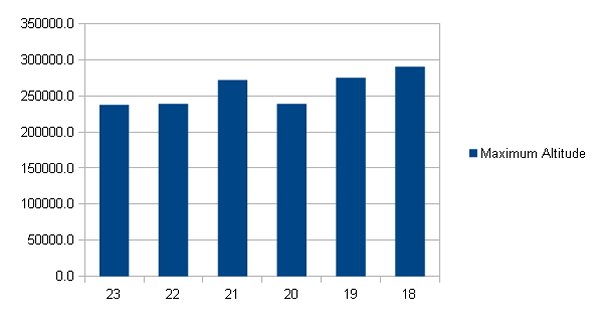
When this code is run under gfortran the rocket reaches a maximum altitude of 237,446 feet.
The met_rocket program was re-engineered to emulate the real arithmetic. The re-engineered code is shown here.
The first test of the re-engineered code was to set the number of mantissa bits of the real numbers to the native values of 23 bits for 4-byte reals and 52 bits for 8-byte reals. The program was built and run. Reassuringly, the simulated rocket stll rose to 237.446 feet. The emulation of the real arithmetic by calling subroutines and functions does not affect the result when the precision is not changed.
All of the working real variables in the program are 4-byte reals. The precision of the 4-byte reals was degraded, one bit at a time, and the program was built and run with each precision. The simulated altitude is tabulated and shown graphically below.
|
|
|
Degrading the precision from the native 23 bits to 22 bits causes a small (0.6%) change in performance. Degrading it to 21 or fewer bits causes significant change (At 21 bits the height changes by 14.6%). It seems that the 23-bit precision of the native 4-byte real numbers is only just sufficient for this simulation program. As a check, the program was converted to run entirely with 8-byte real numbers, with a mantissa of 52 bits. The simulated rocket rose to 237,786 feet. It seems that the (probably accidental) choice of 4-byte real numbers was just good enough.
This result is surprising. The author would have expected a simulation of this type to require 8-byte real numbers. But if 8-byte numbers had been used, and this were a larger, multi-processor simulation, then half of the inter-processor traffic would have been unnecessary.
The program ss_9b.f90 is a nine body simulation of the solar system. The bodies are the Sun and the 8 major planets (Pluto is too small and remote to have much influence on anything else). It models the movements of the bodies and the gravitational forces between them. Again, this is a real program written for a real scientific project.
The code is shown here.
The ss_9b program was re-engineered to emulate the real arithmetic. The re-engineered code is shown here.
The original program and the re-engineered code with an 8-byte precision of 52 bits were both run in a simulation of the orbits for 10 years. The positions of the Sun and of the 8 planets were identical in the two runs. The re-engineering and emulation of the real numbers does not affect the results.
The re-engineered code was then run, progressively reducing the number of bits of precision of the 8-byte real numbers. The radial positions of the first four planets in the plane of the ecliptic are tabulated below (Radii in Astronomical Units - 1 AU is the mean radius of Earth's orbit, angles in degrees).
Mantissa Mercury Venus Earth Mars bits Radius Angle Radius Angle Radius Angle Radius Angle 52 0.4594 -167.91 0.7219 86.70 0.9914 -14.25 1.5899 -123.17 23 0.4596 -167.26 0.7219 86.75 0.9914 -14.17 1.5899 -123.18 22 0.4595 -167.86 0.7219 86.46 0.9914 -14.05 1.5901 -123.15 21 0.4592 -168.96 0.7219 86.67 0.9914 -14.29 1.5901 -123.14 20 0.4600 -165.00 0.7219 84.26 0.9914 -14.36 1.5902 -123.14 19 0.4599 -165.10 0.7219 88.32 0.9914 -14.32 1.5895 -123.29 18 0.4586 -150.26 0.7219 90.00 0.9918 -12.94 1.5907 -122.99 17 0.3222 -17.85 0.7266 52.88 1.0076 -173.43 1.6465 -33.34
Almost nothing changes as the 52-bit precision of the 8-byte numbers is reduced to 23 bits! With only 20 bits of precision the simulation is just beginning to break down. At 17 bits the planets are nowhere near where they should be.
This result was completely unexpected. Again, if this were a multi-processor simulation, half of the inter-processor traffic would be wasted.
There are (at least) two reasons for breakdown of the results of a program as the real number precision is reduced.
The first is excessive numerical drift. No matter what precision is chosen, computations with real numbers contain small errors. As the precision is reduced the relative size of the errors increases, and they cumulate to affect the results. Different expressions and different variables are vulnerable to numerical drift to different extents, because they may depend on different numbers of input variables, and because the errors in the inputs may be correlated. In particular, small differences between large numbers may show this effect.
The second is additive underflow. An IEEE real number is made up of 3 components. A sign bit, an exponent and a mantissa. When two real numbers are added or subtracted, the mantissa of the smaller number is shifted to the right by the number of bits required to make the exponents equal. If the magnitude of one number is very much larger than the other, many of the bits in the smaller number are shifted to the right of the mantissa bits in the result, and are therefore lost in the calculation. The effect is illustrated here.
To find the statements and variables most affected by numerical drift, new statements are automatically inserted into the code to catch the results of all assignments of objects of the native data types (Note that the assignments of user-defined derived types are not captured because the assignment of a derived type must somewhere be preceded by assignment of its components). Assignments of the emulated real types are captured in the same way as the native types. The changes to the code are made automatically by the engineering tool used in this project. The values are captured by calls to subroutines and are written to a binary file, the trace file.
The instrumented code of met_rocket.f is shown here.
The instrumented code of ss_9b.f90 is shown here.
The program is run with native precision, and the trace file of the captured values is created.
The program is re-run repeatedly, reducing the precision of the real numbers progressively. But in the second and subsequent runs, the subroutines which captured the values of the assignments in the first run read the trace file, and compare the values read from the first run with the values which have been computed. When real and complex numbers are compared:
If the numbers are exactly the same, no action is taken;
If the numbers are different, the original number read from the trace file is used to overwrite the number computed. This prevents the accumulation of small differences between the runs;
If the differences between the numbers exceed a criterion value, a report is generated. This indicates a statement in which computation has broken down.
Two criteria are used to compare the values computed with those of the trace file. If the trace file value is below a threshold criterion, no report is made. This prevents the report of large percentage differences when numbers are close to zero. If the trace file value is above the threshold, the percentage difference between the numbers is computed and compared with a criterion percentage.
The calls to the subroutines which write or read the trace file contain a unique integer identifier for the statement in which the assignment was made. This identifier is used to identify the statement at which the program failed.
This technique was first used to eliminate numerical drift from program runs to expose coding errors and compiler bugs. The first major trial was on WRF, the climate and weather modelling code at The University Corporation for Atmospheric Research, Boulder, Colorado and is published here. Note that WRF is a very large program. This technology is scalable.
Additive underflow is detected in the Fortran functions used to overload addition and subtraction of real and complex objects. The code of the check for addition of 4-byte emulated reals is shown here.
The routines which overload addition and subtraction may be called several times in processing a statement. Therefore, the detection of additive underflow is recorded internally when the check is made. It is reported after the statement in the routines which write the results to the trace file.
The results of met_rocket break down when the precision is reduced to 21 bits. The test for excessive numerical drift was made, with a precision of 21 bits, progressively reducing the error criterion until failures were reported. The first failures reported are from a group of statements with the trace labels 210 to 213. The simulation runs for 120,340 time steps and each of these statements is executed once in each time step. The table below shows the number of failures reported for each of these statements in a simulation run with two error criteria. A failure is reported if the result differs from that from the full precision run by more than the criterion percentage.
| Error criterion | |||
|---|---|---|---|
| Code position | 0.00011% | 0.00010% | |
Note the very small percentage errors which occur in these statements. A larger error criterion fails to detect any errors. The statements are:
vel = SQRT(xd*xd+hd*hd) CALL trace_r4_data(vel,210) ! Assume drag is linear with pressure and quadratic with velocity drag = atm_pressure* & (c_drag(2,stage)*vel**2+c_drag(1,stage)*vel) CALL trace_r4_data(drag,211) ! xdd = ((thrust-drag)/mass)*COS(theta) CALL trace_r4_data(xdd,212) hdd = ((thrust-drag)/mass)*SIN(theta)-g CALL trace_r4_data(hdd,213)
The error is in the two acceleration terms, xdd and hdd.
The errors due to additive underflow actually become significant when the precision is reduced to 22 bits. With the error criterion set to 0.1 (i.e. where 10% of the change due to the smaller term is lost) the error counts are shown below:
| Code position | Underflow count | Statement |
|---|---|---|
| vel = SQRT(xd*xd+hd*hd) | ||
| xdd = ((thrust-drag)/mass)*COS(theta) | ||
| hdd = ((thrust-drag)/mass)*SIN(theta)-g | ||
| h = h+frametime*(2*hd-phd) |
The underflow at position 210, the velocity computation, occurs at the maximum height, where the vertical velocity is close to zero.
The underflow at 212 and 213, the thrust-drag computation, occurs at the launch, where the velocity is still very small so the drag is very small.
The underflow at 219 occurs as the maximum height is approached. The change in height is small compared to the height itself so most of the mantissa bits of the change in height are lost. This is the dominant point of failure in the performance with reduced precision.
The solar system simulation, ss_9b starts to break down when the precision is reduced to about 20 bits. The test for excessive numerical drift, with the error ratio criterion set to 1%, shows:
| Code position | Error count |
|---|---|
The code is:
DO axis = 1,3 CALL trace_i4_data(axis,190) ! Difference in position ds(axis,body1,body2) = s(axis,body1)-s(axis,body2) CALL trace_r8_data(ds(axis,body1,body2),191) ! Square of difference in position s2(axis) = ds(axis,body1,body2)*ds(axis,body1,body2) CALL trace_r8_data(s2(axis),192) ENDDO
The error in ds, the difference in position between two bodies, has reached 1%. This is the cause of breakdown of the solar system simulation with decreased precision.
The instrumented code runs very much more slowly than the original code, particularly when run-time trace data are captured to disk. The intention is to use this technique in experiments to identify the precision required for a program, and then to modify the production code to transfer less data between processors, and, if appropriate, to carry out computations at a reduced precision.
It is possible to prove that a given precision, measured in the number of mantissa bits, is sufficient for execution of a given program to a given accuracy.
It is possible to identify the first statements and variables implicated in the breakdown of performance when precision is reduced. The promotion of the precision of specific variables may then free the choice of precisions for less critical variables.
This may have significant implications for packing of data for inter-processor communication in multiprocessor systems.
End of Report